Why Sumproduct?

If you spend much time working with Excel formulas, you’ll start to run into the SUMPRODUCT function a lot. SUMPRODUCT seems to be the catch-all, do-all, go-to solution for many seemingly unrelated Excel problems. Why is SUMPRODUCT in so many Excel formulas?

The main reason SUMPRODUCT appears so often in Excel formulas is that it supports array operations natively, and array operations combined with Boolean logic are a very good way to solve many problems in Excel. In the past (Excel 2019 and older) Excel’s formula engine did not handle most array operations without special handling. As a result, SUMPRODUCT has always been a simple way to create an array formula that “just works”. In the current version of Excel, these limitations are gone , so it is possible to use the SUM function instead.

Note: as mentioned above, the technique of using SUMPRODUCT to solve general problems in Excel often involves some kind of Boolean logic . If this concept is new to you, this video provides a basic overview . The video was created in Excel 365 , so I am using the SUM function, but SUMPRODUCT would work just as well.

The SUMPRODUCT function

The purpose of SUMPRODUCT is to calculate the sum of products. The worksheet below shows a classic example: SUMPRODUCT is used to calculate the sum of Price * Qty:

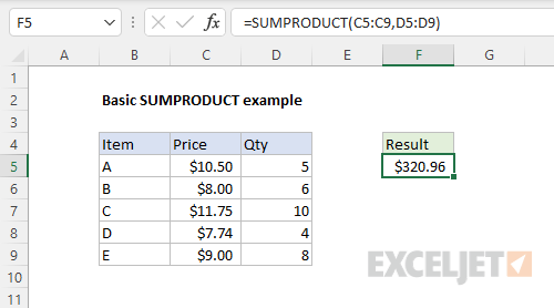
In this worksheet, there is no helper column that calculates the “Extended price” for each item. Instead, SUMPRODUCT calculates the intermediate values by multiplying the two ranges together and returns a sum in one step. Notice we are providing C5:C9 as array1 and D5:D9 as array2 . So far, so good. SUMPRODUCT performs a useful calculation, but there seems to be nothing special about it.

SUMPRODUCT and array operations

In the formula above, we are using two separate arguments , array1 and array2 :

=SUMPRODUCT(C5:C9,D5:D9)

Things get more interesting if we alter the structure of this formula and combine the two arguments into one argument like this:

=SUMPRODUCT(C5:C9*D5:D9)

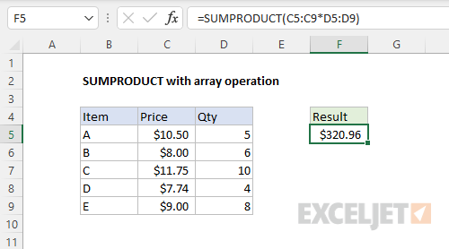
In this formula, we multiply the two ranges together inside array1, using what is called an " array operation “. The formula evaluates like this:

=SUMPRODUCT(C5:C9*D5:D9)
=SUMPRODUCT({10.5;8;11.75;7.74;9}*{5;6;10;4;8})
=SUMPRODUCT({52.5;48;117.5;30.96;72})

After multiplication, there is just one array given to SUMPRODUCT as array1 . The final result is exactly the same as the original formula.

You will see this pattern frequently in SUMPRODUCT — various math operations combined in array1 — because it provides more control over the logic used to manage data. When separate arguments are used, SUMPRODUCT multiplies arguments, which works like AND logic in Boolean algebra . Using one argument means you can use addition (+) for OR logic, or other math operations as needed. As a bonus, any math operation will automatically convert TRUE and FALSE values to 1s and 0s , which are frequently needed to tally up results. Finally, this flexibility means SUMPRODUCT can solve all kinds of tricky problems without Control + Shift + Enter, which is why it’s the go-to function in so many formulas.

A further reason SUMPRODUCT is used so often is that it can handle conditional counts and sums in ways that COUNTIFS and SUMIFS simply can’t. This is because these functions require ranges and can’t use arrays directly. Examples: Count birthdays by year , Sum by year .

The SUM function

In the formula above, notice that we have just a single array after multiplication. When SUMPRODUCT is given one array, it simply returns a sum. In that case, you might wonder if we can replace the SUMPRODUCT function with the SUM function like this:

=SUM(C5:C9*D5:D9)

The answer is: it depends. In modern versions of Excel that include the new dynamic array engine , you can indeed use SUM instead of SUMPRODUCT. However, in older versions of Excel, the SUM version of the formula must be entered as an array formula with Control + Shift + Enter. If not, the formula returns an incorrect result:

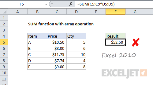
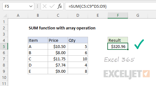
In older versions of Excel (2010, 2016, 2019), the SUM version of the formula returns an incorrect result when the formula is entered normally. In Excel 365, the formula works just fine:

Why does the formula work in SUMPRODUCT but not SUM? Recall that multiplying the two ranges together is an " array operation “. It turns out that SUMPRODUCT is in a small group of functions that can handle most array operations natively. The SUM function is not in this group and must be entered with Control + Shift + Enter when arguments include array operations.

Note: in the example above, we are using just one argument . When only one argument is provided, both SUM and SUMPRODUCT return a sum. With more than one argument, SUM and SUMPRODUCT have different behaviors. SUM returns a sum, while SUMPRODUCT returns the sum of products.

The past

The main reason SUMPRODUCT appears so often in Excel formulas is that it supports array operations natively, and array operations combined with Boolean logic turn out to be a very good way to solve many problems in Excel. In the past (Excel 2019 and older) Excel’s formula engine did not handle most array operations without special handling. As a result, SUMPRODUCT has always been a simple way to create an array formula that “just works”.

In the past, you could use the SUM function instead of SUMPRODUCT in formulas that use array operations, but SUM required Control + Shift + Enter. This means if someone forgets to use CSE when checking or adjusting a formula, the result might change, even if the formula did not change. SUMPRODUCT avoids this problem. It also avoids the need to explain Control + Shift + Enter, which is a complicated topic.

The present

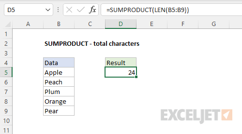
Since dynamic array formulas were introduced in Excel 365 , the need for SUMPRODUCT has started to diminish, because array formulas are natively supported. This means you can replace the SUMPRODUCT function with the SUM function in formulas that use an array operation and get the same behavior. To illustrate with another example, the worksheet below uses the LEN function to count the total number of characters in the range B5:B9.

=SUMPRODUCT(LEN(B5:B9))

Because the range contains five cells, the LEN function returns an array with five counts:

LEN(B5:B9) // returns {5;5;4;6;4}

This is another kind of array operation called lifting . The array from LEN is returned to SUMPRODUCT as array1 :

=SUMPRODUCT({5;5;4;6;4}) // returns 24

And SUMPRODUCT returns 24 as a final result. This formula needs no special handling; it will work in any version of Excel.

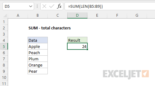
In “modern” versions of Excel, the SUM version of the formula works exactly the same way:

=SUM(LEN(B5:B9))

However, in Legacy Excel the SUM version fails. The screen below shows the same formula in Excel 2010:

=SUM(LEN(B5:B9))

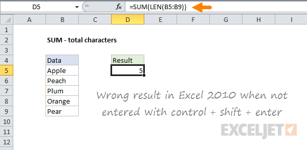
Note that curly braces are not visible in the formula bar. This confirms the formula was not entered with CSE . Below is the same formula, this time entered with Control + Shift + Enter:

{=SUM(LEN(B5:B9))}

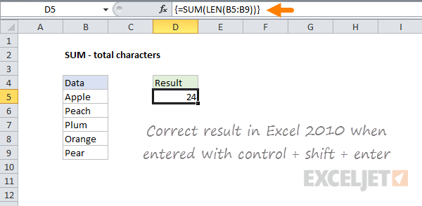
Now the formula returns a correct result. The curly braces in the formula bar confirm the formula was entered with Control + Shift + Enter.

Note: the curly braces are added by Excel automatically when a formula is entered as an array formula with Control + Shift + Enter. Do not add curly braces manually or the formula will not work.

Automatic array formula conversion

To prevent formulas from breaking in older versions of Excel, Excel will automatically convert array formulas to use the array syntax*. This means you will see curly braces in the formula bar even when a formula was never entered with Control + Shift + Enter. For example, the SUM formula above will appear like this if opened in Excel 2016:

{=SUM(LEN(B5:B9))}

Note this is automatic behavior to prevent the formula from returning a different result in older versions of Excel. If the formula is re-entered without Control + Shift + Enter in an older version of Excel, the formula will return an incorrect result.

• Excel is quite conservative in how it evaluates array formulas and you will sometimes see curly braces added to formulas that work just fine without them. For example, you will see the curly braces added to a SUMPRODUCT formula that uses array operations, even when they are not needed. The only way to be sure if the array syntax is needed is to re-enter the formula normally and check the result.

Summary

SUMPRODUCT is in a small group of functions that can handle array operations natively, without Control + Shift + Enter. By placing various operations into a single argument, you can extract data with other functions, and use Boolean algebra to create AND and OR logic in many different ways. This has made SUMPRODUCT the go-to solution for tricky problems over the years.

In Excel 365 and Excel 2021 the formula engine handles arrays natively . This means you can often use the SUM function in place of SUMPRODUCT with the same result and no need to enter the formula in a special way. However, if the same formula is opened in an earlier version of Excel, it will require Control + Shift + Enter.

If you need compatibility with older versions of Excel, SUMPRODUCT is a safer and more robust option, since it “just works” in almost all cases. If you will only be using a worksheet in modern versions of Excel (with the new dynamic array engine ), the SUM function can be used instead of SUMPRODUCT and will work just fine. If you are not sure what version of Excel a worksheet will be used with, SUMPRODUCT is probably the better option, since it avoids complexity.

More Examples

The formulas below use SUMPRODUCT for compatibility with older versions of Excel, but you can use the SUM function instead in modern Excel.

• Count if row meets internal criteria
• Count birthdays by year
• Count cells equal to case sensitive
• Count cells that begin with

Workbook note

The attached workbook below contains the examples used in the article above. Keep in mind that if you open this workbook in older versions of Excel, you will see that the formulas with array operations have already been converted to array formulas. Look for the curly braces in the formula bar, and notice they disappear if you edit the formula. To see the formula fail without this special handling, re-enter the formula normally (i.e. don’t use Control + Shift + Enter).

One of the most important operations in Excel formulas is concatenation. In Excel formulas, concatenation is the process of joining one value to another to form a text string . The values being joined can be hardcoded text, cell references, or results from other formulas.

There are two primary ways to concatenate in Excel:

1. Manually with the ampersand operator (&)
2. Automatically with a function like CONCAT or TEXTJOIN

In the article below, I’ll focus first on manual concatenation with the ampersand operator (&), since this should be your go-to solution for basic concatenation problems. Then I’ll introduce the three Excel functions dedicated to concatenation: CONCATENATE, CONCAT, and TEXTJOIN. These functions can make sense when you need to concatenate many values at the same time. As with so many things in Excel, the most important thing is to understand the basics first.

What is concatenation?

Concatenation is the operation of joining values together to form text. For example, to join “A” and “B” together with concatenation, you can use a formula like this:

="A"&"B" // returns "AB"

The ampersand (&) is Excel’s concatenation operator . Unless you are using one of Excel’s concatenation functions, you will always see the ampersand in a formula that performs concatenation. It’s important to understand that the result from concatenation is always text, even when concatenation involves numbers. For example:

="A"&100 // returns "A100"
=100&200 // returns "100200"

Both of the formulas above return text values, even though some of the values being joined are numeric. In fact, you can transform a number to text by concatenating an empty string (””) to the number like this:

=100&"" // returns "100"

You will sometimes see this technique in a lookup formula that involves numbers and text . Notice in all examples above, text values appear in double quotes (""), while numeric values are not quoted. For example, while 100 is a numeric value, “100” is a text value.

Basic concatenation formula

To explain how concatenation works in a formula in a worksheet, let’s start with a simple example that shows how to concatenate a text string to a value in a cell. With the value 10 in cell B5, this formula will return “Cell B5 contains 10”:

="Cell B5 contains "&B5

There are three things to note in the formula above:

1. The text is enclosed in double quotes ("")
2. The ampersand joins the text and cell B5
3. The cell reference (B5) is not enclosed in quotes

In brief, hardcoded text values are enclosed in double quotes, while cell references, math operators, and function names are not enclosed in quotes.

Now let’s extend the text message above to add a period (.) at the end. In the screen below, the formula in D5 is:

="Cell B5 contains "&B5&"."

In the new formula above, notice two things:

1. We need another ampersand (&) to add the period
2. The period is text and needs to be enclosed in quotes ("")

Naturally, this is a regular Excel formula that will recalculate automatically. If we change the value in B5 to 15, the new result is “Cell B5 contains 15.”.

This example shows the basics of concatenation in Excel with the ampersand (&) operator. Now let’s look at an example of concatenation with some basic formula logic to customize a message.

Concatenation with conditional logic

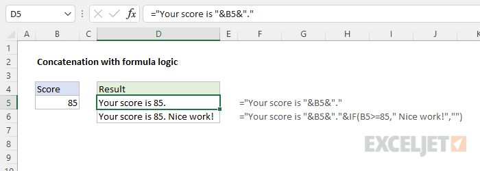
There’s nothing special about concatenation, so you can mix in conditional formula logic as needed. In the formula below, we’re using the same basic structure as the example above, with a different message:

="Your score is "&B5&"."

We start the message, concatenate the value from B5, and concatenate the period. Now let’s extend the formula with some conditional logic. Suppose we want to add the text “Nice work!” to the end of the message when the score is 85 or greater. To do this, we can add the IF function like this:

="Your score is "&B5&"."&IF(B5>=85," Nice work!","")

This looks complicated, so let’s break it into parts. Part 1 is the same as before:

="Your score is "&B5&"." // part 1

Part 2 adds conditional logic based on the IF function:

IF(B5>=85," Nice work!","") // part 2

If the score in cell B5 is 85 or higher, IF returns " Nice work!". Otherwise, IF returns an empty string (""). The final formula simply concatenates part 1 to part 2:

="Your score is "&B5&"."&IF(B5>=85," Nice work!","")

Notice we need another ampersand (&) to join part 1 and part 2, since IF is a function name. Also notice that we have included a space (" “) at the start of " Nice work!” so that this text doesn’t run into the period*. The screen below shows how the two formulas compare:

*Note: in more complex formulas that involve concatenation, you will find you frequently need to adjust space or punctuation to keep the message legible.

Concatenation with number formatting

One tricky aspect of concatenation in Excel is number formatting . Number formats in Excel are a powerful way to control the display of numeric values, but they are not part of the number. This means that number formatting will be lost when you concatenate a formatted number. For example, in the worksheet below, B5 contains 99 formatted with the Currency number format. However, when B5 is concatenated in the formula in D5:

="The price is "&B5

the Currency formatting is lost:

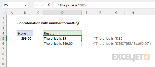
You can add number formatting during concatenation by using the TEXT function in your formula. The formula in D6 is:

="The price is "&TEXT(B5,"$#,##0.00")

In this formula, we place the number in B5 inside the TEXT function and provide a basic Currency number format. As a result, the number 99 is displayed as $99.00 in the result.

Date formatting

Dates are also numbers in Excel and their display is controlled by Date number formatting:

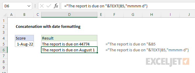
In the worksheet below, the formula in D5 is:

="The report is due on "&B5

Notice the date appears as a raw numeric value . The formula in D5 uses the TEXT function to apply a date format during concatenation:

="The report is due on "&TEXT(B5,"mmmm d")

Excel provides a large number of number formats you can use with the TEXT function. For more details, see Excel custom number formats .

Functions for concatenation

Up to now, we’ve focused on manual concatenation with the ampersand (&) operator. In this section, we’ll look at the functions Excel provides to help with concatenation: CONCATENATE , CONCAT , and TEXTJOIN . In general, CONCATENATE and CONCAT are alternatives to manual concatenation with the ampersand (&) operator, while TEXTJOIN provides more advanced options for working with multiple values. I personally use the ampersand (&) operator as a default approach, and only use the functions below when needed.

CONCATENATE function

The CONCATENATE function is an older function now replaced by the CONCAT function. CONCATENATE allows you to perform simple concatenation only. The values to concatenate and any delimiters are supplied as separate arguments , as seen in the example below:

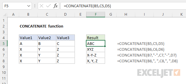
The main benefit of the CONCATENATE function is that values are supplied as separate arguments, with no need for an ampersand (&). The formulas in F5:F8 are:

=CONCATENATE(B5,C5,D5)
=CONCATENATE(B6,C6,D6)
=CONCATENATE(B7,"-",C7,"-",D7)
=CONCATENATE(B8,", ",C8,", ",D8)

Note that hardcoded text values must still be enclosed in double quotes (""), just like manual concatenation with the & operator.

CONCAT function

The CONCAT function replaces the CONCATENATE function in newer versions of Excel. The big difference between the two functions is that CONCAT will accept a range of values:

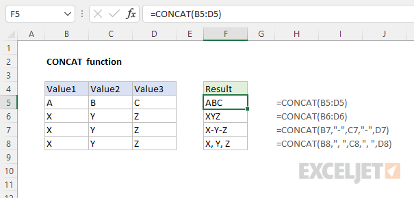
The formulas in F5:F8 are:

=CONCAT(B5:D5)
=CONCAT(B6:D6)
=CONCAT(B7,"-",C7,"-",D7)
=CONCAT(B8,", ",C8,", ",D8)

Notice the first two formulas supply a range directly to CONCAT as a single argument. The ability to provide a range is the primary advantage of CONCAT over CONCATENATE. The next two formulas supply individual values because they are joining values with a delimiter – a hyphen ("-) in the first formula and a comma with a space (", “) in the second formula. Although CONCAT can handle a range, there is no way to provide a delimiter as a separate argument. For this, we need to use the TEXTJOIN function.

TEXTJOIN function

Finally, there is the TEXTJOIN function . Like the CONCAT function, TEXTJOIN is able to accept a range or array of values to concatenate. However, TEXTJOIN provides two additional features that make it especially useful:

1. Ability to accept custom delimiter
2. Ability to ignore empty values

The syntax for TEXTJOIN is:

=TEXTJOIN (delimiter, ignore_empty, text1, [text2], ...)

The first argument, delimiter , is the delimiter to use when joining values. The second argument, ignore_empty , is a Boolean that indicates whether TEXTJOIN should ignore or process empty values. The remaining arguments, text1 , text2 , etc. represent the values to be joined. The worksheet below shows TEXTJOIN in action:

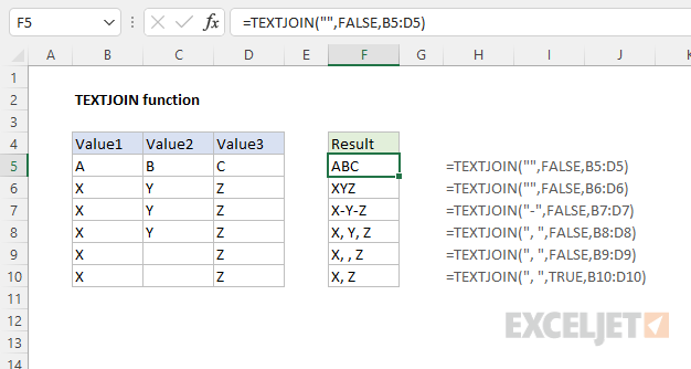
The formulas in F5:F10 are:

=TEXTJOIN("",FALSE,B5:D5)
=TEXTJOIN("",FALSE,B6:D6)
=TEXTJOIN("-",FALSE,B7:D7)
=TEXTJOIN(", ",FALSE,B8:D8)
=TEXTJOIN(", ",FALSE,B9:D9)
=TEXTJOIN(", ",TRUE,B10:D10)

Notice the first two formulas supply an empty string (”") for delimiter , which causes TEXTJOIN to join values directly. The next four formulas all supply one or more characters for delimiter . In cell F9, you can see how the delimiter is repeated when a range contains empty values and ignore_empty is set to FALSE. In F10, ignore_empty has been set to TRUE, and TEXTJOIN ignores the empty value in cell C10.

More examples

Below are more examples that show how concatenation can be used in Excel formulas:

• Join first and last name
• Dynamic worksheet reference
• Count cells greater than
• Make words plural
• Add a line break with a formula

Videos

Here are some videos from our online training that feature concatenation:

• How to join values with the ampersand
• How to use concatenation to clarify assumptions
• Build friendly messages with concatenation