Purpose
Return value
Syntax
=WORKDAY.INTL(start_date,days,[weekend],[holidays])
- start_date - The start date.
- days - Working days before or after start date.
- weekend - [optional] Setting for non-working days.
- holidays - [optional] A list of dates that are non-working days.
Using the WORKDAY.INTL function
The WORKDAY.INTL function calculates a date in the future or past that is a given number of working days from a specified start date, excluding weekends and (optionally) holidays. You can WORKDAY.INTL to calculate project start dates, delivery dates, and completion dates that must ignore non-working days. The WORKDAY.INTL function is more robust than the simpler WORKDAY function because weekend days can be customized so that any day of the week can be a workday or non-workday. Note that WORKDAY.INTL will automatically exclude Saturdays and Sundays but will only exclude holidays if they are provided.
The WORKDAY.INTL function takes four arguments :
- start_date - the date from which to start counting. Note that WORKDAY.INTL does not include the start date as a work day.
- days - the number of days in the future or past to calculate a workday. Use a positive number for days to calculate dates in the future, and a negative number for past dates.
- weekend - an optional argument that controls which days of the week are working and non-working days. If weekend is omitted, WORKDAY.INTL will treat Saturdays and Sundays as non-working days by default. The weekend argument can be provided as a numeric code or a text string like “0000011”. See below for details.
- holidays - an optional argument to provide non-working dates that should be skipped when computing a result. Holidays must be provided as a range or array that contains valid Excel dates.
The WORKDAY.INTL function explained
To illustrate how WORKDAY.INTL works, assume we are scheduling a task that takes 5 working days, starting on Monday, July 1, 2024. The goal is to calculate a date that is 5 working days after July 1, 2024. Beginning with the simplest case, let’s just add 5 days to the start date:
="1-Jul-2024"+5 // returns "6-Jul-2024"
The result is Saturday, July 6, 2024. While this is a valid result, it doesn’t take into account that Saturday is probably not a working day. If, on the other hand, we use WORKDAY.INTL to calculate a date 5 days after July 1:
=WORKDAY.INTL("1-Jul-2024",5) // returns "8-Jul-2024"
The result is Monday, July 8, 2024. This is because WORKDAY.INTL automatically skips Saturdays and Sundays when it calculates a result. Taking things one step further, what if we need to schedule based on a 4-day workweek, where the workdays are Monday through Thursday? In that case, we can extend the formula with the optional weekend argument like this:
=WORKDAY.INTL("1-Jul-2024",5,"0000111") // returns "9-Jul-2024"
The result is now Tuesday, July 9. The text string “0000111” means Mondays, Tuesdays, Wednesdays, and Thursdays are workdays, and Fridays, Saturdays, and Sundays are “weekend days” (i.e. non-working days). Finally, let’s extend the formula one more time and provide two holidays:
=WORKDAY.INTL("1-Jul-2024",5,"0000111",{"4-Jul-2024";"2-Sep-2024"}) // returns "10-Jul-2024"
Since one of the holidays (July 4, 2024) overlaps schedule, WORKDAY.INTL now returns Tuesday, Wednesday, July 10, 2024, since Thursday, July 4, 2024 is also skipped in the calculation.
Note: the holidays above are provided as an array constant but more typically holidays are provided as a range. Remember that holidays must be valid Excel dates. The name of the holiday is not used at all by WORKDAY.INTL.
Of course, in real life, you will not hardcode dates into formulas like this. You will instead use cell references. The screen below shows the four formulas above “ported” to a workbook with cell references. Notice the final calculated date moves farther into the future as we restrict the schedule:
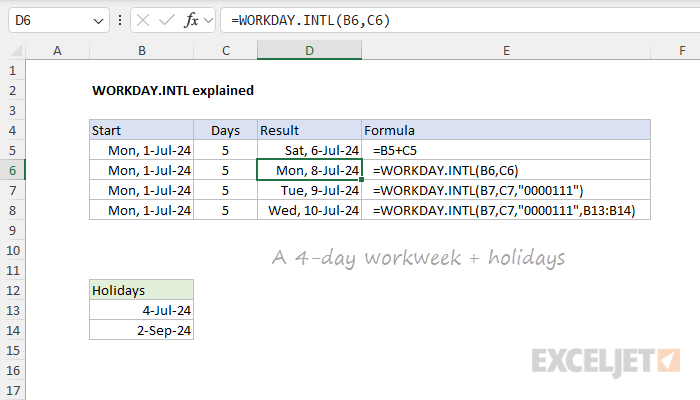
The formula in D5 does not use WORKDAY.INTL and simply adds 5 days to the start date:
=B5+C5 // returns "6-Jul-2024"
The formula in D6 uses the WORKDAY.INTL function but does not provide any holidays:
=WORKDAY.INTL(B6,C6)// returns "8-Jul-2024"
The formula in D7 implements a 4-day workweek by providing “0000111” for the weekend argument:
=WORKDAY.INTL(B7,C7,"0000111") // returns "9-Jul-2024"
Finally, the formula in D8 sets the same 4-day workweek and provides a small list of holidays in B13:B14:
=WORKDAY.INTL(B7,C7,"0000111",B13:B14) // returns "10-Jul-2024"
In all cases, the start_date in column B and the days in column D are the same.
The weekend argument
What makes WORKDAY.INTL different from the original WORKDAY function is the weekend argument. Whereas the WORKDAY function is hardcoded to treat Saturday and Sunday as weekend (i.e. non-working) days the weekend argument in WORKDAY.INTL can be configured to specify any day of the week as a working or non-working day.
The name “weekend” is somewhat confusing since it suggests “end of the week” been when non-working days may occur anywhere in a week, so I recommend you think of the weekend argument in WORKDAY.INTL to mean “non-working days”. This is a more accurate reflection of its purpose.
There are two ways to configure the weekend argument:
- Use a numeric code to select from a pre-configured list of working and non-working days
- Provide a 7-digit code string that provides a setting for every day of the week.
Let’s look at both approaches.
Numeric code for weekend
The first way to provide a value for weekend is to provide a numeric code from the table below , which contains 14 preconfigured options. For example, the generic formulas below show how WORKDAY.INTL can be configured to find the “next” working day with three different workweeks:
- A standard 5-day workweek with Saturday and Sunday as weekend days (1, the default)
- A 5-day workweek with Sunday and Monday as weekend days (2)
- A 6-day workweek with Sundays only as a weekend (11)
=WORKDAY.INTL(A1,1,1) // Saturday and Sunday (default)
=WORKDAY.INTL(A1,1,2) // Sunday and Monday
=WORKDAY.INTL(A1,1,11) // Sunday only
In the last two examples above, we use the numeric code 11 to set weekends to Sundays only. See the table below for the full list of available codes. Note that unlike the “code string” option explained below, these codes are numeric and should not be entered as text. For simplicity, none of the formulas above provided holidays, but they can be added as the fourth argument.
| Code | Weekend days |
|---|---|
| 1 (default) | Saturday, Sunday |
| 2 | Sunday, Monday |
| 3 | Monday, Tuesday |
| 4 | Tuesday, Wednesday |
| 5 | Wednesday, Thursday |
| 6 | Thursday, Friday |
| 7 | Friday, Saturday |
| 11 | Sunday only |
| 12 | Monday only |
| 13 | Tuesday only |
| 14 | Wednesday only |
| 15 | Thursday only |
| 16 | Friday only |
| 17 | Saturday only |
Code string for weekends
The second way to provide a value for weekend is to provide 7-digit text string that covers all seven days of the week, Monday through Saturday. This text string can contain only 1s and 0s. In this scheme, a 1 indicates a weekend (non-working) day, and a 0 indicates a workday. The table below shows sample weekend codes in column B and the workdays they define in column J:

In the image above, shaded cells indicate non-working days and unshaded cells are working days.
The most confusing thing about this method is that you need to “think backwards”: you are not marking working days with a 1, you are marking non-working days with a 1. The zeros are working days . For example, to specify a 6-day workweek with Sunday only as a nonworking day, you would provide “0000001” (row 8 in the worksheet above):
=WORKDAY.INTL(A1,1,"0000001")
To get the next workday that is a Monday, Wednesday, or Friday, you can use a formula like this:
=WORKDAY.INTL(A1,1,"0101011")
To get the next workday that is a Tuesday or Thursday, you can use a formula like this:
=WORKDAY.INTL(A1,1,"1010111")
You can use this same feature to create a list of weekends only , or a list of sequential Mondays, Wednesdays, and Fridays , or any other combination of weekdays, so long as the pattern repeats each week.
Note: weekend must be entered as a text string surrounded by double quotes (i.e.“0000011”) when using this feature. Personally, I prefer the this second approach because it can handle any combination of working/non-working days and you don’t need to look up an arbitrary numeric code.
Worksheet Example
In the worksheet below, Column B contains a variety of different start dates, column C contains the number of days to use, and “holidays” is the named range F5:F13:
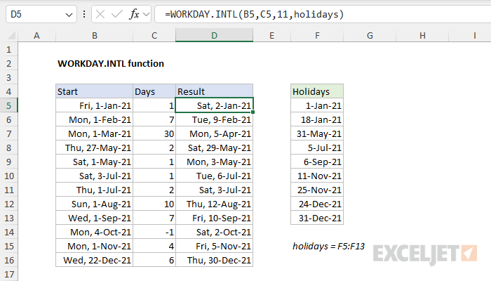
The formula in cell D5 is:
=WORKDAY.INTL(B5,C5,11,holidays)
- start_date - January 1, 2021 (B5)
- days - 1, (C5)
- weekend - 11 (numeric code for Sunday-only weekend)
- holidays - holidays (the named range F5:F13)
As the formula is copied down, WORKDAY.INTL calculates a date n working days from the start date using the value in column C for days . When calculating a result, WORKDAY.INTL excludes dates that are Sundays and dates that are holidays.
Note: named ranges automatically behave like absolute references so there is no need to lock the reference to “holidays” before copying the formula. If you prefer not to use a named range, use an absolute reference like $F$5:$F$13 instead.
Visualized Example
It can be hard to visualize how WORKDAY.INTL works when it calculates a result. The worksheet below contains a more detailed example that shows non-working days shaded in gray in columns D and E:
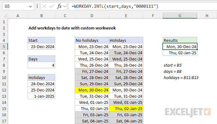
In the example above, WORKDAY.INTL is used to calculate a date that is 4 working days after 23-Dec-2024. The weekend argument is provided as “0000111, " specifying a 4-day workweek where Fridays, Saturdays, and Sundays are non-working days. The formulas in G5 and G6 show the result with and without the holidays in B11:B13:
=WORKDAY.INTL(start,days,"0000111")
=WORKDAY.INTL(start,days,"0000111",holidays)
The first formula (G5) excludes weekend days only and returns December 30, 2024. The second formula (G6) excludes weekend days and holidays and returns January 2, 2025. The dates in columns D and E are not required in this solution, they exist only to help visualize how the WORKDAY.INTL function evaluates working and non-working days and arrives at a final result. The shading and highlighting are applied with conditional formatting . For a full explanation with details, see this page .
Example - is this date a workday?
One problem you might run into is how to test a date to determine whether it is a workday. You can use WORKDAY.INTL for this task, but the formula is not immediately obvious. Essentially, we need to “trick” WORKDAY.INTL into evaluating a given date by shifting the date back one day and then asking for the next workday. You can see this approach in the worksheet below. The formula in cell D5 is:
=WORKDAY.INTL(B5-1,1,"0000111",holidays)=B5
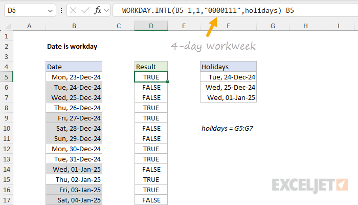
For a more detailed explanation, see this example: Date is Workday .
Recommendations
- Use cell references for the start date, days, and holidays to make it easy to adjust the output quickly.
- Using the code string format for weekend (e.g. “0000111”) is more flexible than a numeric code because you can make any day of the week a workday or non-workday.
- WORKDAY.INTL returns a date. If you need to calculate the number of working days between two dates, see the NETWORKDAYS function or the more flexible NETWORKDAYS.INTL function .
Notes
- WORKDAY.INTL returns a date that is a given number of working days from a specified start_date
- WORKDAY.INTL does not include the start date as a work day.
- Use a positive number for days to calculate dates in the future, and a negative number for past dates.
- If any argument is invalid, WORKDAY.INTL will return #NUM! or #VALUE!, depending on the input.
- If days is zero, WORKDAY.INTL will return the start_date unchanged.
- The weekend argument can be provided as a numeric code or a text string like “0000011”
- Holidays must be provided as valid Excel dates in a range or array.
Purpose
Return value
Syntax
=YEAR(date)
- date - A valid Excel date.
Using the YEAR function
The YEAR function returns the year of a date as a 4-digit number. YEAR takes just one argument, date , which must be a valid date. Date can be a cell containing a date, a date string, or a formula that returns a date. Internally, Excel converts dates to serial numbers following its own date system. For example, given the date “23-Aug-2012”, YEAR will return 2021:
=YEAR("23-Aug-2012") // returns 2012
Note: dates are serial numbers in Excel, and begin on January 1, 1900. Dates before 1900 are not supported.
Key features
Returns year as 4-digit number (e.g., 2024, not 24)
Works with any valid Excel date
Often combined with DATE, MONTH, DAY for date manipulation
Returns a number, not a text value
Can accept dates as text strings, cell references, or formulas
Basic examples
Get year from date
Add years to date
Get fiscal year from date
Count dates in given year
Sum by year
Year is a leap year
Notes
Basic examples
The YEAR function requires just one argument, which must be a valid date or a value that Excel can convert into a valid date. With the date January 20, 2026, in cell A1, the following formula will return 2026:
=YEAR(A1) // returns 2026
Note that you can use YEAR to extract the year from a date entered as text:
=YEAR("1/20/2026") // returns 2026
However, using text for dates can cause unpredictable results on computers using different regional date settings. In general, it’s better to supply a reference to a cell that already contains a valid date.
You can easily combine the YEAR function with other Excel functions. For example, to get the current year, you can use YEAR with the TODAY function like this:
=YEAR(TODAY()) // returns current year
Using the DATE function , you can extract a year from cell A1 and use it to create the date January 1 in the same year, like this:
=DATE(YEAR(A1),1,1) // first day of same year
If A1 contains January 20, 2026, the result will be January 1, 2026.
Get year from date
Use the DATE function to extract just the year from a date. In the worksheet below, the formula in D5 is:
=YEAR(B5)
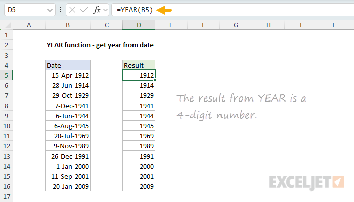
The YEAR function takes just one argument, the date from which you want to extract the year. With a date value for 15-Apr-1912 in B5, the YEAR function returns the number 1912. For more details, see Get year from date .
Add years to date
In this example, the goal is to add a given number of years to a date. The formula in E5 is:
=DATE(YEAR(B5)+C5,MONTH(B5),DAY(B5))
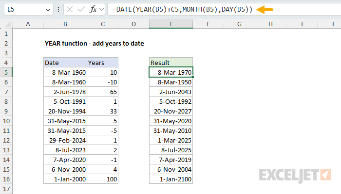
This formula uses the DATE function together with the YEAR, MONTH, and DAY functions. Working from the inside out, YEAR, MONTH, and DAY “take apart” the date into separate components. The DATE function then reassembles the date, adding the number in C5 to the year value along the way. With the date 8-Mar-1960 in B5, and the number 10 in C5, the result is 8-Mar-1970.
Another approach is to use the EDATE function . For more details, see Add years to date .
Get fiscal year from date
The YEAR function only returns a normal year number, not a fiscal year. However, you can get YEAR to return a fiscal year by combining it with the MONTH function. You can see this approach below, where the fiscal year starts in July. The formula in D5 is:
=YEAR(B5)+(MONTH(B5)>=7)
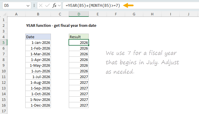
By convention, a fiscal year is denoted by the year in which it ends. So if a fiscal year begins in July, then July 1, 2026 is in fiscal year 2027, while June 1, 2026 is in fiscal year 2026. The YEAR function first extracts the year from the date. Then, a boolean expression is added to adjust for the fiscal year:
+(MONTH(B5)>=7) // returns 0 or 1
If the month is greater than or equal to 7 (July), the expression returns TRUE, which Excel evaluates as 1. This increments the year by one. If the month is less than 7, the expression returns FALSE (zero), and the year remains unchanged.
For more details, see Get fiscal year from date .
Count dates in given year
In this example, the goal is to count how many dates fall in a given year. The formula in E5 is:
=SUMPRODUCT(--(YEAR(dates)=D5))
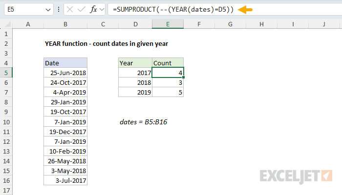
The YEAR function extracts the year from each date in the named range dates (B5:B16). Because B5:B16 contains 12 cells, YEAR returns an array of 12 year values. This array is compared to the year in D5, creating a new array of TRUE and FALSE values.
The double negative (–) converts the TRUE/FALSE values to 1s and 0s. Finally, SUMPRODUCT sums the array, returning a count of dates that match the year.
This pattern of using Boolean logic in array operations is powerful and flexible, and is also used with functions like FILTER and XLOOKUP .
For more details, see Count dates in given year .
Sum by year
In this example, the goal is to calculate a total for each year. All data is in an Excel Table named “data”. The formula in G5 is:
=SUMPRODUCT((YEAR(data[Date])=F5)*data[Amount])
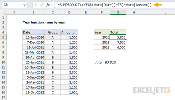
Working from the inside out, the YEAR function extracts year values from the dates in the data table. These year values are compared to the year in F5, creating an array of TRUE and FALSE values. This array is multiplied by the amounts, which converts TRUE/FALSE to 1/0 and effectively “cancels out” amounts from other years. SUMPRODUCT then sums the resulting array to return the total for the year.
For more details, see Sum by year .
Year is a leap year
Excel doesn’t have a function to test for a leap year. However, you can roll your own by combining several functions together. In the worksheet below, the goal is to test whether the year of a date is a leap year for all dates in column B. The formula in D5 is:
=MONTH(DATE(YEAR(B5),2,29))=2
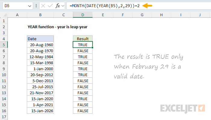
This formula exploits a behavior of the DATE function. When you request February 29 in a non-leap year, DATE automatically rolls forward to March 1. The YEAR function extracts the year from the date, and DATE constructs a date for February 29 of that year. Then the MONTH function is used to test the month number of the resulting date. If the month is 2 (February), it’s a leap year (TRUE). If the month is 3 (March), it’s not a leap year (FALSE).
Note: Excel incorrectly treats 1900 as a leap year due to a legacy bug from Lotus 1-2-3. To guard against this, you can add an AND condition: =AND(MONTH(DATE(YEAR(B5),2,29))=2,YEAR(B5)<>1900)
For more details, see Year is a leap year .
Notes
- YEAR returns a #VALUE! error if the date argument is not a valid date.
- Dates before January 1, 1900 are not supported in Excel’s date system.
- The result is a number, not text. To display just the year from a date, you can apply a custom number format like “yyyy”.
- YEAR can accept dates entered as text strings (e.g., “1/5/2016”), but this can cause issues with different regional date settings.
- Excel incorrectly treats 1900 as a leap year due to a legacy bug inherited from Lotus 1-2-3.
Explanation
Working from the inside out, EDATE first calculates a date 6 months in the future. In the example shown, that date is December 24, 2015.
Next, the formula subtracts 1 day to get December 23, 2015, and the result goes into the WORKDAY function as the start date, with days = 1, and the range B9:B11 provided for holidays.
WORKDAY then calculates the next business day one day in the future, taking into account holidays and weekends.
If you need more flexibility with weekends, you can use WORKDAY.INTL.
Explanation
In the worksheet shown, column B contains 12 dates. The goal is to calculate the next working day after each date, taking into account weekends (Saturday and Sunday) and the holidays listed in column F. In other words, the formula should automatically skip weekends and any dates defined as non-working days.
WORKDAY function
The WORKDAY function takes a date and returns the next working day n days in the future or past. You can use WORKDAY to calculate things like ship dates, delivery dates, and completion dates that need to take into account working and non-working days. The generic syntax for WORKDAY looks like this:
=WORKDAY(start_date,days,[holidays])
Where days is a number (n) and holidays is an optional range that contains non-working dates. For this problem, we want the next working day, so we provide 1 for days . The formula in D5, copied down, looks like this:
=WORKDAY(B5,1,holidays)
Where holidays is the named range F5:F15, which contains days that should be excluded. The WORKDAY function is fully automatic. Given a valid date, it will add days to the date, skipping weekends and holidays. Named ranges behave like absolute references by default, so the range will not change as the formula is copied down. Without a named range, you will need to lock the reference like this:
=WORKDAY(B5,1,$F$5:$F$15)
As the formula is copied down, it returns the next business day after the starting date in column B. Saturdays and Sundays are automatically skipped, as well as any dates that appear in the range F5:F15.
Current date or next workday
There may be situations where you want to return the current date when it’s a working day or the next working date if not. To do this, you can adjust the formula like so:
=WORKDAY(B5-1,1,holidays)
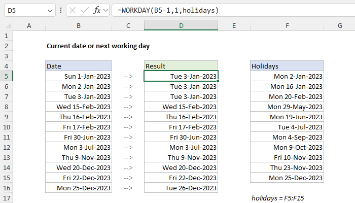
Here, we first subtract 1 day from the date inside the WORKDAY function, then feed that date to WORKDAY as the start_date . WORKDAY then moves forward one day to the original date and checks the result. If the original date is a working day, WORKDAY returns the date unchanged. Otherwise, WORKDAY will continue to move forward one day at a time, skipping weekends and holidays along the way, until it finds a valid workday. You can see the result in the worksheet above.
Custom weekends
The WORKDAY function defines a weekend as Saturday and Sunday only. If you need more flexibility on which days of the week are considered weekends or working days, use the WORKDAY.INTL function instead. For example, to calculate the next working day for this example with a standard work week of Monday-Thursday, where weekend days are Friday, Saturday, and Sunday, you can use WORKDAY.INTL like this:
=WORKDAY.INTL(B5,1,"0000111",holidays)
WORKDAY.INTL includes an extra argument called weekend that can be provided as a string of 1s and 0s like “0000111”. In this scheme, a 1 indicates a weekend and a 0 indicates a workday. For more details, see How to use the WORKDAY.INTL function .
