Purpose
Return value
Syntax
=YEAR(date)
- date - A valid Excel date.
Using the YEAR function
The YEAR function returns the year of a date as a 4-digit number. YEAR takes just one argument, date , which must be a valid date. Date can be a cell containing a date, a date string, or a formula that returns a date. Internally, Excel converts dates to serial numbers following its own date system. For example, given the date “23-Aug-2012”, YEAR will return 2021:
=YEAR("23-Aug-2012") // returns 2012
Note: dates are serial numbers in Excel, and begin on January 1, 1900. Dates before 1900 are not supported.
Key features
Returns year as 4-digit number (e.g., 2024, not 24)
Works with any valid Excel date
Often combined with DATE, MONTH, DAY for date manipulation
Returns a number, not a text value
Can accept dates as text strings, cell references, or formulas
Basic examples
Get year from date
Add years to date
Get fiscal year from date
Count dates in given year
Sum by year
Year is a leap year
Notes
Basic examples
The YEAR function requires just one argument, which must be a valid date or a value that Excel can convert into a valid date. With the date January 20, 2026, in cell A1, the following formula will return 2026:
=YEAR(A1) // returns 2026
Note that you can use YEAR to extract the year from a date entered as text:
=YEAR("1/20/2026") // returns 2026
However, using text for dates can cause unpredictable results on computers using different regional date settings. In general, it’s better to supply a reference to a cell that already contains a valid date.
You can easily combine the YEAR function with other Excel functions. For example, to get the current year, you can use YEAR with the TODAY function like this:
=YEAR(TODAY()) // returns current year
Using the DATE function , you can extract a year from cell A1 and use it to create the date January 1 in the same year, like this:
=DATE(YEAR(A1),1,1) // first day of same year
If A1 contains January 20, 2026, the result will be January 1, 2026.
Get year from date
Use the DATE function to extract just the year from a date. In the worksheet below, the formula in D5 is:
=YEAR(B5)
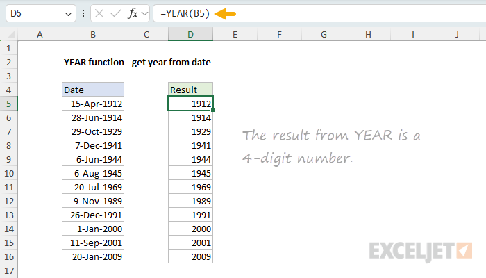
The YEAR function takes just one argument, the date from which you want to extract the year. With a date value for 15-Apr-1912 in B5, the YEAR function returns the number 1912. For more details, see Get year from date .
Add years to date
In this example, the goal is to add a given number of years to a date. The formula in E5 is:
=DATE(YEAR(B5)+C5,MONTH(B5),DAY(B5))
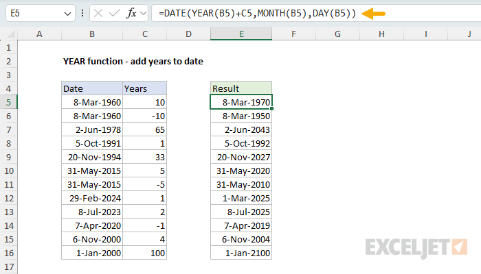
This formula uses the DATE function together with the YEAR, MONTH, and DAY functions. Working from the inside out, YEAR, MONTH, and DAY “take apart” the date into separate components. The DATE function then reassembles the date, adding the number in C5 to the year value along the way. With the date 8-Mar-1960 in B5, and the number 10 in C5, the result is 8-Mar-1970.
Another approach is to use the EDATE function . For more details, see Add years to date .
Get fiscal year from date
The YEAR function only returns a normal year number, not a fiscal year. However, you can get YEAR to return a fiscal year by combining it with the MONTH function. You can see this approach below, where the fiscal year starts in July. The formula in D5 is:
=YEAR(B5)+(MONTH(B5)>=7)
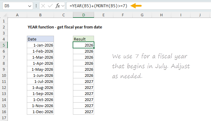
By convention, a fiscal year is denoted by the year in which it ends. So if a fiscal year begins in July, then July 1, 2026 is in fiscal year 2027, while June 1, 2026 is in fiscal year 2026. The YEAR function first extracts the year from the date. Then, a boolean expression is added to adjust for the fiscal year:
+(MONTH(B5)>=7) // returns 0 or 1
If the month is greater than or equal to 7 (July), the expression returns TRUE, which Excel evaluates as 1. This increments the year by one. If the month is less than 7, the expression returns FALSE (zero), and the year remains unchanged.
For more details, see Get fiscal year from date .
Count dates in given year
In this example, the goal is to count how many dates fall in a given year. The formula in E5 is:
=SUMPRODUCT(--(YEAR(dates)=D5))
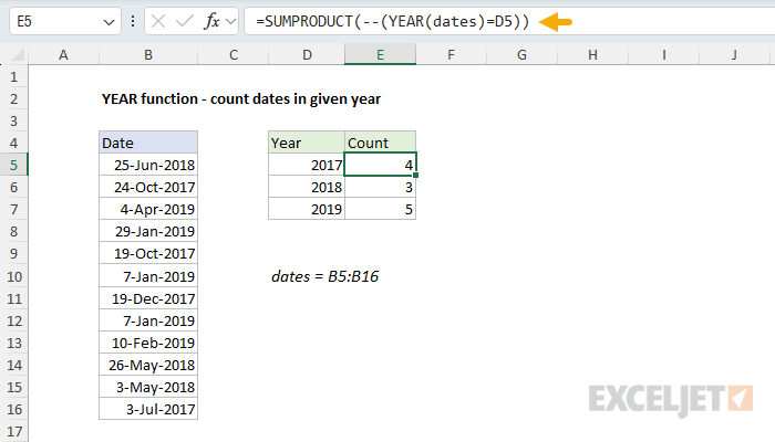
The YEAR function extracts the year from each date in the named range dates (B5:B16). Because B5:B16 contains 12 cells, YEAR returns an array of 12 year values. This array is compared to the year in D5, creating a new array of TRUE and FALSE values.
The double negative (–) converts the TRUE/FALSE values to 1s and 0s. Finally, SUMPRODUCT sums the array, returning a count of dates that match the year.
This pattern of using Boolean logic in array operations is powerful and flexible, and is also used with functions like FILTER and XLOOKUP .
For more details, see Count dates in given year .
Sum by year
In this example, the goal is to calculate a total for each year. All data is in an Excel Table named “data”. The formula in G5 is:
=SUMPRODUCT((YEAR(data[Date])=F5)*data[Amount])
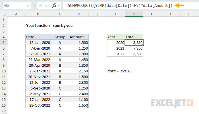
Working from the inside out, the YEAR function extracts year values from the dates in the data table. These year values are compared to the year in F5, creating an array of TRUE and FALSE values. This array is multiplied by the amounts, which converts TRUE/FALSE to 1/0 and effectively “cancels out” amounts from other years. SUMPRODUCT then sums the resulting array to return the total for the year.
For more details, see Sum by year .
Year is a leap year
Excel doesn’t have a function to test for a leap year. However, you can roll your own by combining several functions together. In the worksheet below, the goal is to test whether the year of a date is a leap year for all dates in column B. The formula in D5 is:
=MONTH(DATE(YEAR(B5),2,29))=2
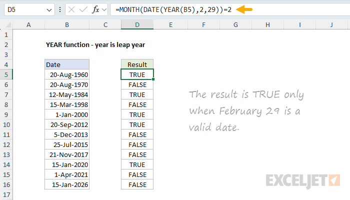
This formula exploits a behavior of the DATE function. When you request February 29 in a non-leap year, DATE automatically rolls forward to March 1. The YEAR function extracts the year from the date, and DATE constructs a date for February 29 of that year. Then the MONTH function is used to test the month number of the resulting date. If the month is 2 (February), it’s a leap year (TRUE). If the month is 3 (March), it’s not a leap year (FALSE).
Note: Excel incorrectly treats 1900 as a leap year due to a legacy bug from Lotus 1-2-3. To guard against this, you can add an AND condition: =AND(MONTH(DATE(YEAR(B5),2,29))=2,YEAR(B5)<>1900)
For more details, see Year is a leap year .
Notes
- YEAR returns a #VALUE! error if the date argument is not a valid date.
- Dates before January 1, 1900 are not supported in Excel’s date system.
- The result is a number, not text. To display just the year from a date, you can apply a custom number format like “yyyy”.
- YEAR can accept dates entered as text strings (e.g., “1/5/2016”), but this can cause issues with different regional date settings.
- Excel incorrectly treats 1900 as a leap year due to a legacy bug inherited from Lotus 1-2-3.
Purpose
Return value
Syntax
=YEARFRAC(start_date,end_date,[basis])
- start_date - The start date.
- end_date - The end date.
- basis - [optional] The type of day count basis to use (see below).
Using the YEARFRAC function
YEARFRAC returns a decimal number representing years between two dates. For example:
=YEARFRAC("1-Jan-2019","1-Jan-2020") // returns 1
=YEARFRAC("1-Jan-2019","1-Jul-2020") // returns 1.5
=YEARFRAC("1-Jan-2019","1-Jan-2021") // returns 2
Although the generic syntax for YEARFRAC shows the start date followed by the end date, you can provide the dates in any order with the same result. For example:
=YEARFRAC("1-Jan-2000","1-Jan-2019") // returns 19
=YEARFRAC("1-Jan-2019","1-Jan-2000") // returns 19
Basis options
YEARFRAC uses whole days between two dates to calculate the fraction of a year as a decimal number. The YEARFRAC function accepts an optional argument called “basis” that controls how days are counted when computing fractional years. The default behavior is to count days between two dates based on a 360-day year, where all 12 months are considered to have 30 days. The table below summarizes the available options:
| Basis | Calculation | Notes |
|---|---|---|
| 0 (default) | 30/360 | US convention |
| 1 | actual/actual | |
| 2 | actual/360 | |
| 3 | actual/365 | |
| 4 | 30/360 | European convention |
Note that basis 0 (the default) and basis 4 both operate based on a 360-day year, but they handle the last day of the month differently. With the US convention, when the start date is the last day of the month, it is set to the 30th day of the same month. When the end date is the last day of the month, and the start date < 30, the end date is set to the 1st of the next month, otherwise the end date is set to the 30th of the same month. With the European convention, start dates and end dates equal to the 31st of a month are set to the 30th of the same month.
Examples
With a start date in cell A1, and an end date in cell B1, the YEARFRAC will return years between the two dates as a decimal number:
=YEARFRAC(A1,B1) // years between two dates
To get a whole number only (not rounded), you can use the INT function like this:
=INT(YEARFRAC(A1,B1)) // whole number only, discard decimal
To get current age based on a birthdate, you can use a formula like this:
=INT(YEARFRAC(birthdate,TODAY())) // age from birthdate
Note: this formula can sometimes return incorrect results. See this example for more details.
To get the percentage of the current year complete, you can use YEARFRAC like this:
=YEARFRAC(DATE(YEAR(TODAY()),1,1),TODAY()) // % year complete
Full explanation here .
